Define morphological models with neat.PhysTree

The Class neat.PhysTree is used to define the physiological parameters of neuron models. It inherits from neat.MorphTree and thus has all its functionality. Just as neat.MorphTree, instances are initialized based on the standard .swc format:

from neat import PhysTree
ph_tree = PhysTree('morph/L23PyrBranco.swc')

              -- N E S T --
  Copyright (C) 2004 The NEST Initiative

 Version: 3.8.0-post0.dev0
 Built: Apr 15 2025 08:54:20

 This program is provided AS IS and comes with
 NO WARRANTY. See the file LICENSE for details.

 Problems or suggestions?
   Visit https://www.nest-simulator.org

 Type 'nest.help()' to find out more about NEST.

Defining physiological parameters

A PhysTree consists of neat.PhysNode instances, which inherit from neat.MorphNode. Compared to a MorphNode, a PhysNode has extra attributes (initialized to some default value) defining physiological parameters:

# specific membrance capacitance (uF/cm^2)
print('default c_m node 1:', ph_tree[1].c_m)
# axial resisitance (MOhm*cm)
print('default r_a node 1:', ph_tree[1].r_a)
# point-like shunt located at {'node': node.index, 'x': 1.} (uS)
print('default g_shunt node 1:', ph_tree[1].g_shunt)
# leak and ion channel currents, stored in a dict with
# key: 'channel_name', value: [g_max, e_rev]
print('default currents node 1:', ph_tree[1].currents)

default c_m node 1: 1.0
default r_a node 1: 9.999999999999999e-05
default g_shunt node 1: 0.0
default currents node 1: {}

It is not recommended, and for ion channels even forbidden, to set the parameters directly via the nodes. Rather, the parameters should be specified with associated functions of PhysTree. These functions accept a node_arg keyword argument, which allows selecting a specific set of nodes. Parameters, can be given as float, in which case all nodes in node_arg will be set to the same value, a dict of {node.index: parameter_value}, or a callable function where the input is the distance of the middle of the node (loc = {'node': node.index, 'x': .5}) to the soma and the output the parameter.

Let’s use PhysTree.set_physiology() to set capacitance (1st argument) and axial resistance (2nd argument) in the whole tree:

ph_tree.set_physiology(lambda x: .8 if x < 60. else 1.6*.8, 100.*1e-6)

Here, we defined the capacitance to be \(.8\) \(\mu\)F/cm\(^2\) when the mid-point of the node is less than 60 \(\mu\)m from the soma and \(1.6*.8\) \(\mu\)F/cm\(^2\), a common factor to take dendritic spines into account. Axial resistance was set to a constant value throughout the tree.

To set ion channels (see the ‘Ionchannels in NEAT’ tutorial on how to create your own ion channels), we must create the ion channel instance first. Here, we’ll set a default sodium and potassium channel:

from channelcollection_for_tutorial import Na_Ta, Kv3_1
# create the ion channel instances
na_chan = Na_Ta()
k_chan = Kv3_1()
# set the sodium channel only at the soma, with a reversal of 50 mV
ph_tree.add_channel_current(na_chan, 1.71*1e6, 50., node_arg=[ph_tree[1]])
# set the potassium channel throughout the dendritic tree, at 1/10th
# of its somatic conductance, and with a reversal of -85 mV
gk_soma = 0.45*1e6
ph_tree.add_channel_current(k_chan, lambda x: gk_soma if x < .1 else gk_soma/10., -85.)

Now, we only have to set the leak current. We have two possibilities for this: (i) we could set the leak current by providing conductance and reversal in the standard way with PhysTree.set_leak_current() or (ii) with could fit the leak current to fix equilibrium potential and membrane time scale (if possible) with PhysTree.fit_leak_current(). We take the second option here:

# fit leak current to yield an equilibrium potential of -70 mV and
# a total membrane time-scale of 10 ms (with channel opening
# probabilities evaluated at -70 mV)
ph_tree.fit_leak_current(-70., 10.)

Inspecting the physiological parameters

We can now inspect the contents of various PhysNode instances:

# soma node
print(ph_tree[1])

PhysNode 1, Parent: None --- r_a = 0.0001 MOhm*cm, c_m = 0.8 uF/cm^2, v_ep = -70 mV, (g_Na_Ta = 1.71e+06 uS/cm^2, e_Na_Ta = 50 mV), (g_Kv3_1 = 450000 uS/cm^2, e_Kv3_1 = -85 mV), (g_L = 31.5408 uS/cm^2, e_L = -48.6388 mV)

# dendrite node
print(ph_tree[115])

PhysNode 115, Parent: 114 --- r_a = 0.0001 MOhm*cm, c_m = 1.28 uF/cm^2, v_ep = -70 mV, (g_Kv3_1 = 45000 uS/cm^2, e_Kv3_1 = -85 mV), (g_L = 123.193 uS/cm^2, e_L = -69.4148 mV)

Or, to get the full information on conductances and reversal potentials of membrane currents:

# soma node
print(ph_tree[1].currents)

{'Na_Ta': [1710000.0, 50.0], 'Kv3_1': [450000.0, -85.0], 'L': [31.5408107318479, -48.638804987272735]}

# dendrite node
print(ph_tree[115].currents)

{'Kv3_1': [45000.0, -85.0], 'L': [123.19344287327353, -69.41475491536458]}

Active dendrites compared to closest passive version

Imagine we aim to investigate the role of active dendritic channels, and to that purpose want to compare the active dendritic tree with a passive version. We may compute the leak conductance of this “passified” tree as the sum of all ion channel conductance evaluate at the equilibrium potential. The equilibrium potentials is stored on the tree using PhysTree.set_v_ep():

ph_tree.set_v_ep(-70.)

To obtain the passified tree, we use PhysTree.as_passive_membrane(). However, this function will overwrite the parameters of the original nodes, if we want to maintain the initial tree, we have to copy it first:

# copy the initial tree
ph_tree_pas = PhysTree(ph_tree)
# set to passive (except the soma)
ph_tree_pas.as_passive_membrane(node_arg=[n for n in ph_tree_pas if n.index != 1])

We can now inspect the nodes:

# soma node
print(ph_tree_pas[1])

PhysNode 1, Parent: None --- r_a = 0.0001 MOhm*cm, c_m = 0.8 uF/cm^2, v_ep = -70 mV, (g_Na_Ta = 1.71e+06 uS/cm^2, e_Na_Ta = 50 mV), (g_Kv3_1 = 450000 uS/cm^2, e_Kv3_1 = -85 mV), (g_L = 31.5408 uS/cm^2, e_L = -48.6388 mV)

# dendrite node
print(ph_tree_pas[115])

PhysNode 115, Parent: 114 --- r_a = 0.0001 MOhm*cm, c_m = 1.28 uF/cm^2, v_ep = -70 mV, (g_L = 128 uS/cm^2, e_L = -70 mV)

And the currents:

# soma node
print(ph_tree_pas[1].currents)

{'Na_Ta': [1710000.0, 50.0], 'Kv3_1': [450000.0, -85.0], 'L': [31.5408107318479, -48.638804987272735]}

# dendrite node
print(ph_tree_pas[115].currents)

{'L': [128.00000000000003, -70.0]}

Comparing this to the previously shown nodes of the full tree, we see that the dendrite nodes have been “passified”.

Computational tree

The computational tree in PhysTree works the same as in MorphTree, except that it’s derivation also considers changes in physiological parameters, next to changes in morphological parameters.

ph_tree.set_comp_tree()
# compare number of nodes in computational tree and original tree
print('%d nodes in original tree'%(len(ph_tree)))
with ph_tree.as_computational_tree:
    print('%d nodes in computational tree'%(len(ph_tree)))

432 nodes in original tree
98 nodes in computational tree

Compare this to the number of nodes in the computational tree induced solely by the morphological parameters:

from neat import MorphTree
m_tree = MorphTree('morph/L23PyrBranco.swc')
m_tree.set_comp_tree()
with m_tree.as_computational_tree:
    print('%d nodes in computational `MorphTree`'%len(m_tree))

87 nodes in computational `MorphTree`

Note: only call this PhysTree.set_comp_tree when all physiological parameters have been set, and never change parameters stored at individual nodes when the computational tree is active, as this leads to the computational tree being inconsistent with the original tree.

Preparing NEAT models for simulation

To simulate models from NEAT, we first need to compile the ion channels. NEAT’s IonChannel class instances can generate their own code for .mod files or .nestml files, which are then compiled into either NEURON or NEST. For this purpose, NEAT provides the neatmodels terminal command, which should be invoked as follows to prepare the models for this tutorial:

neatmodels install TutorialChannels -s neuron nest -p channelcollection_for_tutorial.py

All installed models can be visualized with neatmodels list -s neuron nest, and can also be uninstalled (i.e. neatmodels uninstall {model name} -s {simulator}).

Installed models can then be loaded with into e.g. NEURON.

from neat import load_neuron_model
load_neuron_model('TutorialChannels')

Simulating NEAT models in NEURON

NEAT implements an interface to the NEURON simulator, so that models defined by neat-trees can be simulated with the NEURON simulator. To have access to this functionality, the NEURON simulator and it’s Python interface need to be installed.

The class neat.NeuronSimTree implements this interface, and inherits from neat.PhysTree. Hence, a NeuronSimTree can be defined in the same way as a PhysTree.

from neat import NeuronSimTree
sim_tree = NeuronSimTree('morph/L23PyrBranco.swc')
sim_tree.set_physiology(lambda x: .8 if x < 60. else 1.6*.8, 100.*1e-6)
# ... etc

Copying trees

If a different type of tree is needed than the one originally defined, or simply a copy of the original tree, we can use the copy construct functionality of NEAT’s trees: we can instantiate any tree class based on any other tree instance, and only the attributes that are shared amongst both instances will be copied over. Since NeuronSimTree is a subclass of PhysTree, we end up with an identical tree, but with additional functions and associated attributes to simulate the associated NEURON model.

sim_tree = NeuronSimTree(ph_tree)

First, we must initialize the tree structure into hoc.

sim_tree.init_model(t_calibrate=100.)

We may then add inputs to the tree. NEAT implements a number of standard synapse types and current injections. Let’s apply a DC current step to the soma and also give some input to a conductance-based dendritic synapse.

# somatic DC current step with amplitude = 0.100 nA, delay = 5. ms and duration = 50. ms
sim_tree.add_i_clamp((1.,.5), 0.010, 5., 50.)
# dendritic synapse with rise resp. decay times of .2 resp 3. ms and reversal of 0 mV
sim_tree.add_double_exp_synapse((115,.8), .2, 3., 0.)
# give the dendritic synapse a weight of 0.005 uS and connect it to an input spike train
sim_tree.set_spiketrain(0, 0.005, [20.,22.,28.,29.,30.])

We will record voltage at the somatic and dendritic site. Recording locations should be stored under the name ‘rec locs’.

sim_tree.store_locs([(1,.5), (115,.8)], name='rec locs')

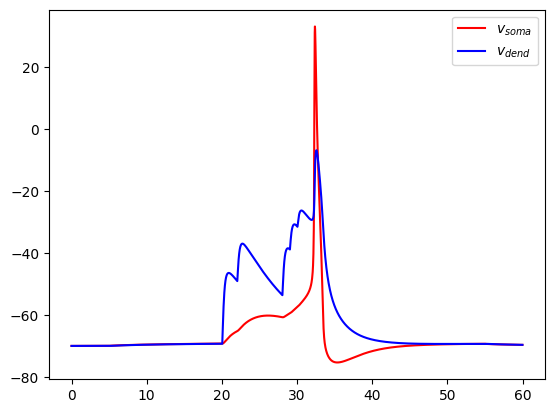
We can then run the model for \(60\) ms and plot the results:

# simulate the model and delete all hoc-variables afterwards
res = sim_tree.run(60.)
sim_tree.delete_model()

# plot the results
import matplotlib.pyplot as pl
pl.plot(res['t'], res['v_m'][0], c='r', label=r'$v_{soma}$')
pl.plot(res['t'], res['v_m'][1], c='b', label=r'$v_{dend}$')
pl.legend(loc=0)
pl.show()

User defined point-process

Note that it is very easy to add user defined point-process to the NeuronSimTree. In fact, all any of the default functions to add point-process do, is defining a neat.MorphLoc based on the input, so that the point process is added at the right coordinates no matter whether the original or computational tree was active. All hoc sections are stored in the dict self.sections which has as keys the node indices. Hence, in pseudo code one would do:

loc = neat.MorphLoc((node.index, x-coordinate), sim_tree)

# define the point process at the correct location
pp = h.user_defined_point_process(sim_tree.sections[loc['node']](loc['x']))

# set its parameters
pp.param1 = val1
pp.param2 = val2
...

# store the point process (e.g. if it is a synapse in `sim_tree.syns`)
sim_tree.syns.append(pp)

Evaluate impedance matrices with neat.GreensTree

The class neat.GreensTree inherits from neat.PhysTree and implements Koch’s algorithm [-@Koch1984] to calculate impedances in the Fourrier domain. For a given input current of frequency \(\omega\) at location \(x\), the impedance gives the linearized voltage response at a location \(x^{\prime}\): \begin{align} v_{x^{\prime}}(\omega) = z_{x^{\prime}x}(\omega) \, i_x(\omega). \end{align} Applying the inverse Fourrier transform yields a convolution in the the time domain: \begin{align} v_{x^{\prime}}(t) = z_{x^{\prime}x}(t) \ast i_x(t), \end{align} with we call \(z_{x^{\prime}x}(t) = FT^{-1} \left( z_{x^{\prime}x}(\omega) \right)\) the impedance kernel. The steady state impedance is then: \begin{align} z_{x^{\prime}x} = \int_0^{\infty} \mathrm{d}t \, z_{x^{\prime}x}(t) = z_{x^{\prime}x}(\omega = 0). \end{align}

Computing an impedance kernel

To compute an impedance kernel, we first have to initialize the GreensTree:

from neat import GreensTree
greens_tree = GreensTree(ph_tree)

For the calculation to proceed efficiently, GreensTree first sets effective, frequency-dependent boundary conditions for each cylindrical section. Hence we must specify the frequencies at which we want to evaluate impedances. If we aim to also compute temporal kernels, neat.FourierQuadrature is a handy tool to obtain the correct frequencies. Suppose for instance that we aim to compute an impedance kernels from \(0\) to \(50\) ms:

from neat import FourierQuadrature
import numpy as np
# create a FourierQuadrature instance with the temporal array on which to evaluate the impedance kernel
t_arr = np.linspace(0.,50.,1000)
ft = FourierQuadrature(t_arr)
# appropriate frequencies are stored in `ft.s`
# set the boundary condition for cylindrical segments in `greens_tree`
greens_tree.set_impedance(ft.s)

We can now compute for instance the impedance kernel between dendritic and somatic site:

z_trans = greens_tree.calc_zf((1,.5), (115,.8))

# plot the kernel
pl.plot(ft.s.imag, z_trans.real, 'b')
pl.plot(ft.s.imag, z_trans.imag, 'r')
pl.xlim((-1000.,1000.))
pl.show()

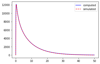
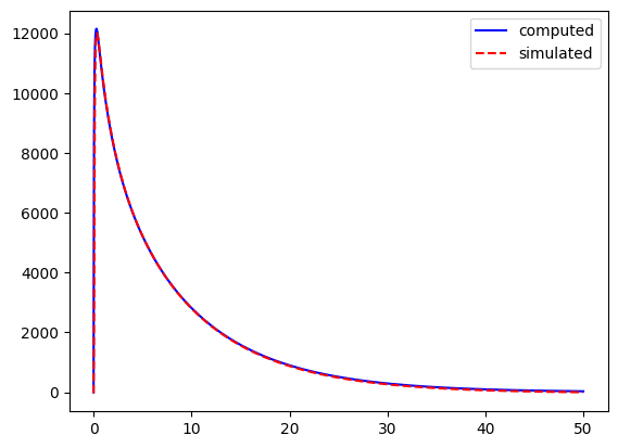
We can also obtain this kernel in the time domain with the FourierQuadrature object:

# time domain kernel
tt, zt = ft.ft_inv(z_trans)

# comparison with NEURON simulation
sim_tree.init_model(t_calibrate=300.)
i_amp, i_dur = 0.001, 0.1
sim_tree.add_i_clamp((115,.8), i_amp, 0., i_dur)
res = sim_tree.run(50.)
sim_tree.delete_model()
res['v_m'] -= res['v_m'][:,-1]
res['v_m'] /= (i_amp*1e-3*i_dur)

# plot the kernel
pl.plot(tt, zt.real, 'b', label='computed')
pl.plot(res['t'], res['v_m'][0], 'r--', label='simulated')
pl.legend(loc=0)
pl.show()

Computing the impedance matrix

While GreensTree.calc_zf() could be used to explicitely compute the impedance matrix, GreensTree.calc_impedance_matrix() uses the symmetry and transitivity properties of impedance kernels to further optimize the calculation.

z_locs = [(1,.5), (115,.8)]
z_mat = greens_tree.calc_impedance_matrix(z_locs)

This matrix has shape (len(ft.s), len(z_locs), len(z_locs)). The zero-frequency component is at ft.ind_0s. Hence, the following gives the steady state impedance matrix:

print(z_mat[ft.ind_0s])

[[ 88.07091747+0.j  83.93186356+0.j]
 [ 83.93186356+0.j 183.59769195+0.j]]

Simplify a model with neat.CompartmentFitter

The class neat.CompartmentFitter is used to obtain simplified compartmental models, where the parameters of the compartments are optimized to reproduce voltages at any set of locations on the morphology. It is initialized based on a neat.PhysTree:

from neat import CompartmentFitter
c_fit = CompartmentFitter(ph_tree)

>>>> Cache file for CompartmentFitter:
    neatcache/_cache_b80d98f3e873c5a168e383cad92be3706ce4673e3ef50cd55b9e66529d75e49a.p
<<<<

The function CompartmentFitter.fit_model() then returns a neat.CompartmentTree object defining the simplified model, with the parameters of the optimized compartments:

# compute a simplified tree containing a somatic and dendritic compartment
f_locs = [(1,.5), (115,.8)]
c_tree, c_locs = c_fit.fit_model(f_locs, use_all_channels_for_passive=False)

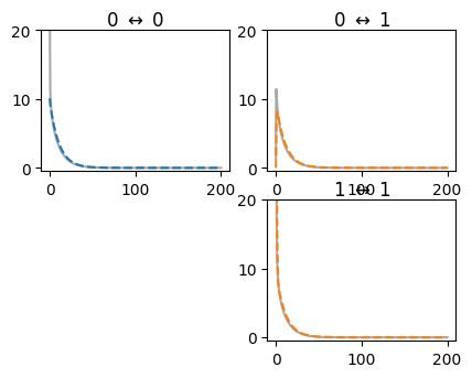
One way to understand whether the reduction will be faithful, is to check whether the passive reduced model reproduces the same impedance kernels as the full model. The check_passive() function of neat.CompartmentFitter allows the comparison of these kernels between full and reduced models:

c_fit.check_passive(f_locs, use_all_channels_for_passive=False)

The simplified model neat.CompartmentTree

Each neat.CompartmentNode in the CompartmentTree stores the optimized parameters of the compartment, and the coupling conductance with it’s parent node.

print(c_tree)

>>> CompartmentTree
    CompartmentNode 0, Parent: None --- loc_idx = 0, g_c = 0.0 uS, ca = 9.914229970918551e-05 uF, e_eq = -70.0000000000006 mV, (g_L = 0.009188301476232499 uS, e_L = -68.82253558506142 mV), (g_Na_Ta = 14.378466892350664 uS, e_Na_Ta = 50.0 mV), (g_Kv3_1 = 7.000477231569277 uS, e_Kv3_1 = -85.0 mV)
    CompartmentNode 1, Parent: 0 --- loc_idx = 1, g_c = 0.009224434868094789 uS, ca = 4.2683265272914205e-06 uF, e_eq = -70.0000000000006 mV, (g_L = 0.00041103448332490333 uS, e_L = -69.71819327183215 mV), (g_Na_Ta = 2.580260653895025e-13 uS, e_Na_Ta = 50.0 mV), (g_Kv3_1 = 0.07229641499492892 uS, e_Kv3_1 = -85.0 mV)

To keep track of the mapping between compartments and locations, each CompartmentNode also has a loc_idx attribute, containing the index of the location in the original list given to CompartmentFitter.fit_model() (here f_locs) to which the compartment is fitted:

# node 0 corresponds to location 0 in `f_locs`
print('node index: %d, loc index: %d'%(c_tree[0].index, c_tree[0].loc_idx))
# node 1 corresponds to location 1 in `f_locs`
print('node index: %d, loc index: %d'%(c_tree[1].index, c_tree[1].loc_idx))

node index: 0, loc index: 0
node index: 1, loc index: 1

Here, these indices correspond, but in general there is no guarantee this will be the case. A list of ‘fake’ locations for the compartmental model can also be obtained. These locations contain nothing but the node index and an x-coordinate without meaning.

c_locs = c_tree.get_equivalent_locs()
print(c_locs[0], c_locs[1])

(0, 0.5) (1, 0.5)

Simulate the simplified model with neat.NeuronCompartmentTree

The simplified model can be simulated directly in NEURON, with the same API as neat.NeuronSimTree. To do so, one can create a neat.NeuronCompartmentTree from an existing neat.CompartmentTree:

from neat import NeuronCompartmentTree
c_sim_tree = NeuronCompartmentTree(c_tree)

We may now check whether our simplification was successful by running the same simulation for the full and reduced models:

# initialize, run and delete the full model, set input locations as stored in `f_locs`
sim_tree.init_model(t_calibrate=100.)
sim_tree.add_i_clamp(f_locs[0], .01, 5., 50.)
sim_tree.add_double_exp_synapse(f_locs[1], .2, 3., 0.)
sim_tree.set_spiketrain(0, 0.002, [20.,22.,28.,28.5,29.,30.,31.])
sim_tree.store_locs(f_locs, name='rec locs')
res_full = sim_tree.run(60.)
sim_tree.delete_model()

# initialize and run the simplified model, set input locations as stored in `c_locs`
c_sim_tree.init_model(t_calibrate=100.)
c_sim_tree.add_i_clamp(c_locs[0], 0.01, 5., 50.)
c_sim_tree.add_double_exp_synapse(c_locs[1], .2, 3., 0.)
c_sim_tree.set_spiketrain(0, 0.002, [20.,22.,28.,28.5,29.,30.,31.])
c_sim_tree.store_locs(c_locs, name='rec locs')
res_reduced = c_sim_tree.run(60.)
# print the hoc topology of the reduced model
from neuron import h
h.topology()
# delete the reduced model
c_sim_tree.delete_model()

|-|       0(0-1)
  `|       1(0-1)

Simulate the simplified model with neat.NestCompartmentTree

The simplified model can also be exported to NEST. To this purpose, we first import NEST and load the NEST model featuring the tutorial channels

import nest
dt = 0.1
nest.ResetKernel()
nest.SetKernelStatus(dict(resolution=dt))

from neat import load_nest_model
load_nest_model("TutorialChannels")

Jun 16 21:59:47 SimulationManager::set_status [Info]:
    Temporal resolution changed from 0.1 to 0.1 ms.

Jun 16 21:59:49 Install [Info]:
    loaded module TutorialChannels_module

We can then use a NestCompartmentTree to translate the NEAT compartment tree to NEST

from neat import NestCompartmentTree
c_tree_nest = NestCompartmentTree(c_tree)
cm = c_tree_nest.init_model("TutorialChannels", 1) # equivalent of nest.Create()

We implement the same stimulation in NEST using NEST-specific simulation control.

# NEST-specific simulation control
# adding receptors
cm.receptors = [
    {
        "comp_idx": 0,
        "receptor_type": "curr_in",
    },
    {
        "comp_idx": 1,
        "receptor_type": "i_AMPA",
        "params": {"e_AMPA": 0.0, "tau_r_AMPA": 0.2, "tau_d_AMPA": 3.0},
    },
]
# connect spike input to i_AMPA receptor
sg = nest.Create("spike_generator", 1, {"spike_times": [20.,22.,28.,28.5,29.,30.,31.]})
nest.Connect(
    sg, cm,
    syn_spec={
        "synapse_model": "static_synapse",
        "weight": 0.002,
        "delay": dt,
        "receptor_type": 1,
    },
)
# connect DC current to curr_in receptor
dc = nest.Create("step_current_generator", 1,
    params={
        "amplitude_times": [5.,50.],
        "amplitude_values": [0.01,0.],
    }
)
nest.Connect(
    dc, cm,
    syn_spec={
        "synapse_model": "static_synapse",
        "weight": 1.0,
        "delay": 0.1,
        "receptor_type": 0,
    }
)
# voltage recording
mm = nest.Create(
    "multimeter",
    1,
    {
        "record_from": ["v_comp0", "v_comp1"],
        "interval": dt,
    },
)
nest.Connect(mm, cm)

# simulate
nest.Simulate(60.0)

res_nest = nest.GetStatus(mm, "events")[0]

Jun 16 21:59:50 NodeManager::prepare_nodes [Info]:
    Preparing 4 nodes for simulation.

Jun 16 21:59:50 SimulationManager::start_updating_ [Info]:
    Number of local nodes: 4
    Simulation time (ms): 60
    Number of OpenMP threads: 1
    Number of MPI processes: 1

Jun 16 21:59:50 SimulationManager::run [Info]:
    Simulation finished.

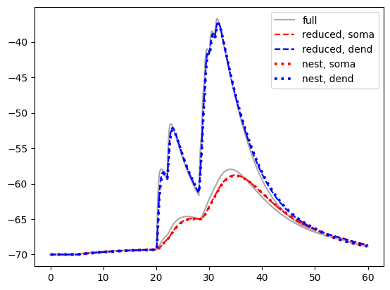
We compare somatic and dendritic voltages in both models:

pl.plot(res_full['t'], res_full['v_m'][0], c='DarkGrey', label='full') # soma full model, NEURON
pl.plot(res_full['t'], res_full['v_m'][1], c='DarkGrey') # dendrite full model, NEURON
pl.plot(res_reduced['t'], res_reduced['v_m'][0], 'r--', lw=1.6, label='reduced, soma') # soma reduced model, NEURON
pl.plot(res_reduced['t'], res_reduced['v_m'][1], 'b--', lw=1.6, label='reduced, dend') # soma reduced model, NEURON
pl.plot(res_nest['times'], res_nest['v_comp0'], 'r:', lw=2.6, label='nest, soma') # soma reduced model, NEST
pl.plot(res_nest['times'], res_nest['v_comp1'], 'b:', lw=2.6, label='nest, dend') # soma reduced model, NEST

pl.legend(loc=0)
pl.show()